
Mastering Postgres indexes in 10 minutes
What’s in this post?
Enough about the insides of Postgres indexes to impress your coworkers at the coffee machine or recruiters at a job interview 🤓.
We’ll have a look at B-Tree, Hash, GIN, GiST, BRIN indexes and focus on demystifying them.
Why the hell do I even need an index?
Indexes are at the core of any querying in relational databases (the classic SQL databases like Postgres or MySQL). Therefore it is very rewarding and important to have an idea of how they work.
An illustration is worth a thousand words so let’s take an example. Let’s say we have a user table containing 1M million entries (or rows):
CREATE TABLE user (
  id   SERIAL PRIMARY KEY,
  name TEXT,
  age  INTEGER
);
We want to know how many of our users are above 30. We run:
SELECT COUNT(*) FROM user WHERE age > 30;
Without any extra index, the database would have to go over the 1M entries one by one, look at their age and increment a counter for all the users above 30:
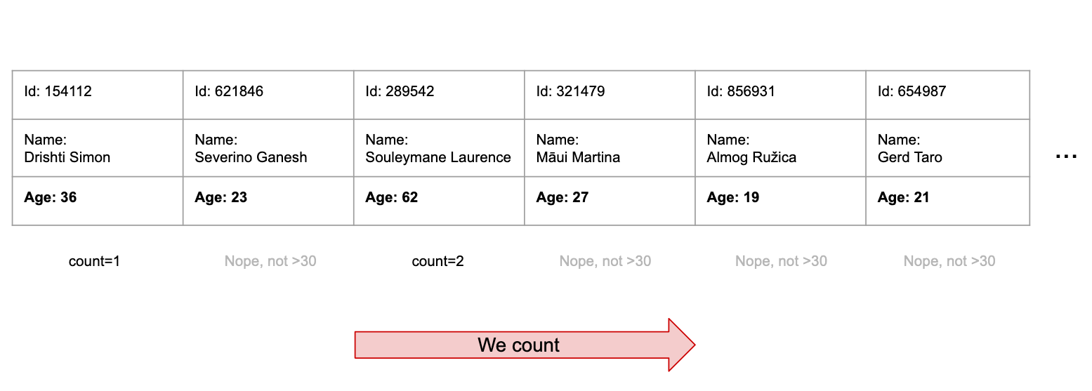
If it feels like an inefficient way of getting the result it’s because it is 💁♀️. It would be a slow query (called a “full table scan”, as every row needs to be scanned).
That’s where indexation comes into play. It will allow us to quickly locate the users we’re interested in, without having to lookup all the rows.
In Postgres, there are 5 types of indexes:
- B-Trees
- Hashes
- GINs
- GiSTs
- BRINs
Before we start
Naming
- Row: An entry in the database (e.g. a user). Also called tuple.
- Column: An attribute of a row (e.g. the first name of a user).
- Table: A collection of rows (e.g. a user table).
- TID: Tuple ID. It’s an internal Postgres ID. It describes where to find the row on the disk.
- Operator: Reserved keyword representing operations on data (e.g.
AND,+,>,=). - Statement: Database operation (e.g.
CREATE TABLE user (name TEXT);). - Query: Statement that returns data (e.g.
SELECT * FROM user;)
Core assumptions
- In general, an index needs to be able to fit in RAM to be fully efficient. That’s why having very large indexes can be problematic.
- Fetching the row behind a
tidis easy and relatively cheap to do. We consider it roughly equivalent to getting an element from an array by index (e.g.var a = array[i]). - We’ll only talk about read operations (queries). How to propagate writes to indexes is a whole other story.
- Everything is more complex and complicated in real life, this post tries to explain things on a very high level and may be approximate on some parts. For more details, one should have a look at the
Further explanationlinks.
B-Tree indexes
Usecase
So we want to index this query. We want to make it faster:
SELECT COUNT(*) FROM user WHERE age > 30;
We create a B-Tree index on the age column.
CREATE INDEX user_by_age ON user (age);
No need to specify anything, B-Tree is the default index for Postgres and many other databases including MySQL, Oracle or SQL Server.
How does it work
A binary search tree (different from a B-Tree) is a well known data structure where every node of the tree has two children nodes. The values of the left and right children being respectively smaller and larger than their parent’s value.
A B-Tree is a generalised binary search tree where every node can have more than two children.
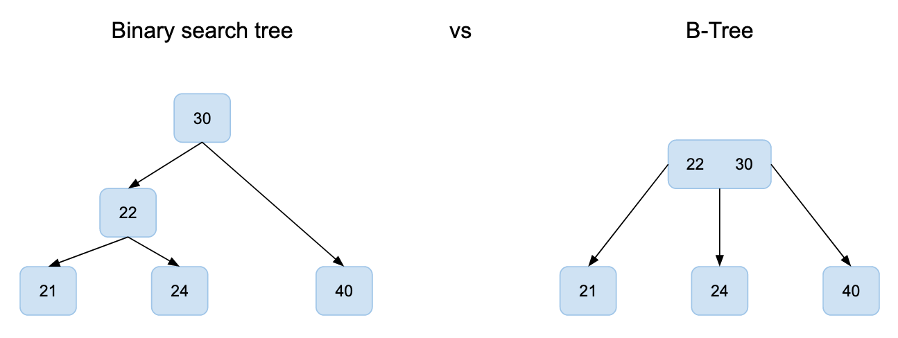
A very helpful property of these trees is that their values are sorted. It makes it easy to lookup values. Exactly what we need to speed up our query!
Now a B-Tree index is slightly more than just a B-Tree. It is a linked list of tids, sorted by value and linked to a B-Tree.
Let’s run our query again and see how it looks like:
SELECT COUNT(*) FROM user WHERE age > 30;
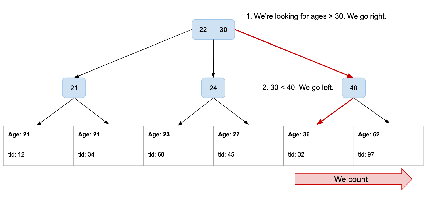
That was much easier! By using the sorting of the tree nodes, we can now quickly find the first user being above 30 and count from there. Remember? The linked list at the bottom is sorted by age!
As a side note, you may be wondering about multicolumn indexes, like:
CREATE INDEX user_by_age_and_height ON user (age, height_cm);
The simplest way to visualize it is to imagine it as being roughly equivalent to a monocolumn index like:
CREATE INDEX user_by_age_and_height ON user (age+'-'+height_cm);
The B-Tree mechanism stays the same, but the values that are being sorted are now for example 28-182.
This explains why the index wouldn’t help with trying to run:
SELECT COUNT(*) FROM user WHERE height_cm > 160;
In the tree, values like 28-182 are not sorted by height. They are sorted by age, and then for every individual age they are sorted by height.
On the other hand, the index would help us with this query:
SELECT COUNT(*) FROM user WHERE age = 30 AND height_cm > 160;
TLDR (Too Long Didn’t Read)
- B-Tree is the default index in many databases.
- Is it so popular because it’s fast, efficient and flexible.
- It makes operations like
=,<,<=,>,>=,ORDER BYor evenLIKEfaster. - A rule of thumb would be: if you need to speed up the above operations, use a B-Tree index unless there is a specific reason not to.
Further explanation
- https://www.qwertee.io/blog/postgresql-b-tree-index-explained-part-1/
- https://habr.com/en/company/postgrespro/blog/443284
Hash indexes
Usecase
We’re only querying using the = operator and we’re having very specific scaling/performance issues (e.g. our table is huge and a B-Tree would be too large to fit in memory). We want to index:
SELECT COUNT(*) FROM user WHERE name = 'Souleymane Laurence';
We create a Hash index on the name column.
CREATE INDEX user_by_name ON user USING HASH (name);
This time, we need to specify it explicitely by adding USING HASH to our statement.
How does it work
Let’s think of our user table as a Java array for one second. We consider the position in the array to be equivalent to a tid in Postgres:
User[] userTable = {...}
That’s how we’d naively lookup the users having the name Souleymane Laurence:
User[] userTable = {...}

int i;
List<int> foundTids = new ArrayList<>();

// Iterating over the rows of our table to find our values in the array.
for (i = 0; i < userTable.length; i++) {
	if (userTable[i].name == "Souleymane Laurence") {
		foundTids.add(i)
	}
}
This is slow because we have to go over all the entries of the table one by one (remember, they could be hundreds of millions in a database).
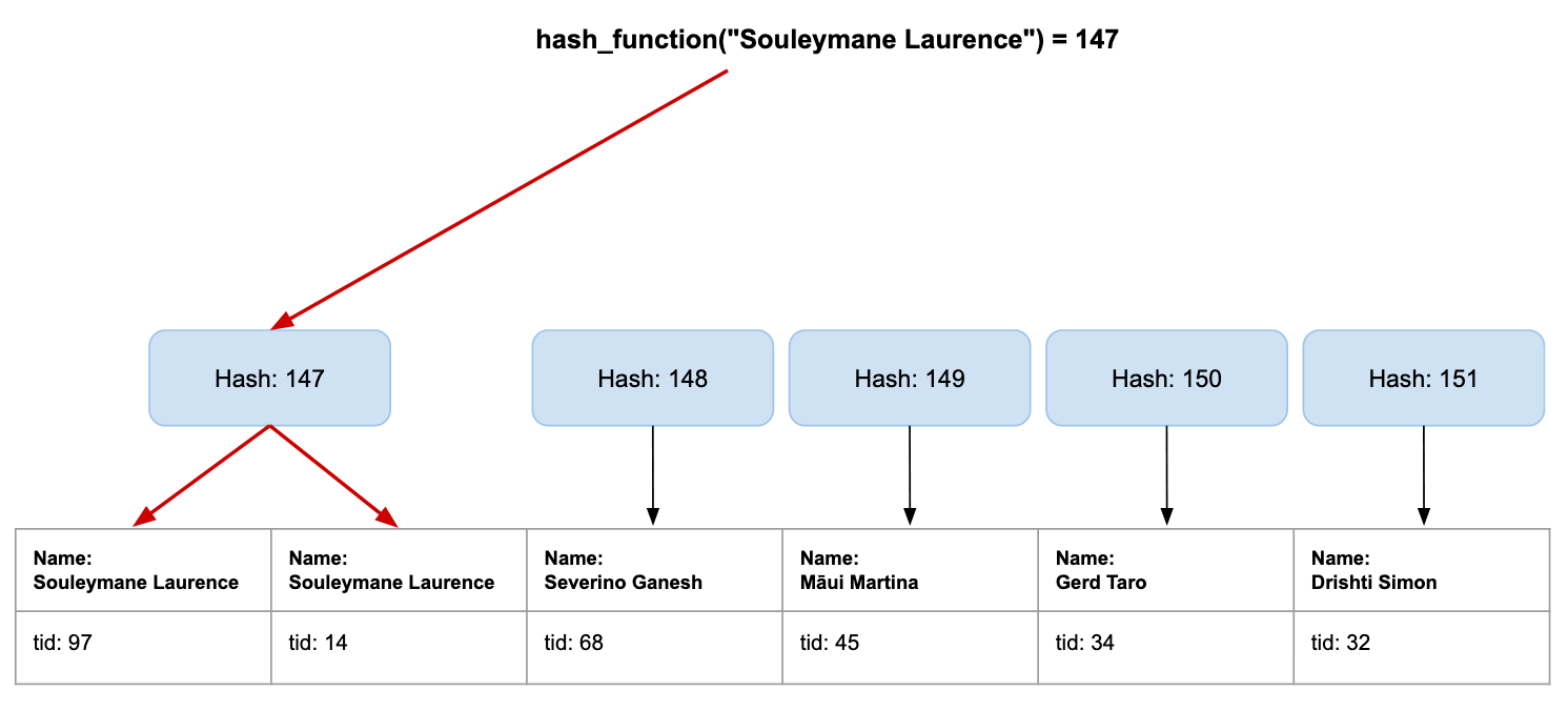
Now couldn’t we find a way to remove this big for loop and predict in advance where are our rows going to be located in the array? Yes! And it’s called a hash function.
A hash function is capable of taking any input and translating it into a smaller subset of values:
// Returns an int between 0 and 256.
// Always the same for the same input.
hash_function_256("Souleymane Laurence")
-> 147
We could use this as an array position! We just need to rearrange our table first:
User[] userTable = {...}

int i;
List<int>[] hashIndex = new List<int>[256]; // 256 hash values

// Iterating over the rows of our table to populate our index.
for (i = 0; i < userTable.length; i++) {
	int hash = hash_function(userTable[i].name)
	hashIndex[hash].add(i)
}
We just created our own hash index. Let’s now run our query again:
// Our new index.
List<int>[] hashIndex = {...}

int hash = hash_function_256("Souleymane Laurence")
List<int> foundTids = hashIndex[hash]
That’s it, and that was quick as hell 🔥. Back to SQL:
SELECT COUNT(*) FROM user WHERE name = 'Souleymane Laurence';
TLDR
- The hash index was never very popular for a few reasons:
- Before Postgres 10, hash indexes were not properly supported. In particular they were not recorded in the write-ahead log so they could not be recovered after a failure/incident.
- They only index the
=operator and also don’t help with sorting. They’re not very flexible and for=, the B-Tree does the job very well too.
- So why should you use a hash index? Probably you shouldn’t. But they are smaller in size and can be faster than B-Trees so they can be useful under certain conditions. The read time being constant (
O(1)vsO(log n)for B-Trees), they could for example be beneficial for a high throughput of lookups by ID on a huge table.
Further explanation
- https://habr.com/en/company/postgrespro/blog/442776
- https://medium.com/@jorsol/postgresql-10-features-hash-indexes-484f319db281
GIN (Generalized Inverted Index)
Usecase
GIN indexes are mostly useful for indexing multi-valued columns (e.g. arrays, full-text search).
Let’s add a favorite_colors column to our users:
ALTER TABLE user ADD COLUMN favorite_colors TEXT[];
We want to be able to index a query that looks up users that have red and blue in their favorite colors:
SELECT COUNT(*) FROM user WHERE favorite_colors @> '{red,blue}';
We now create a GIN index:
CREATE INDEX user_by_favorite_colors ON user USING GIN (favorite_colors);
How does it work
Spoiler alert: GIN indexes are actually custom B-Trees where the multi-valued columns (arrays for example) are flattened 😱. The only difference is that we’re adding a bitmap scan at the end of the operation for multi-value lookups.
Let’s run our query:
SELECT COUNT(*) FROM user WHERE favorite_colors @> '{red,blue}';
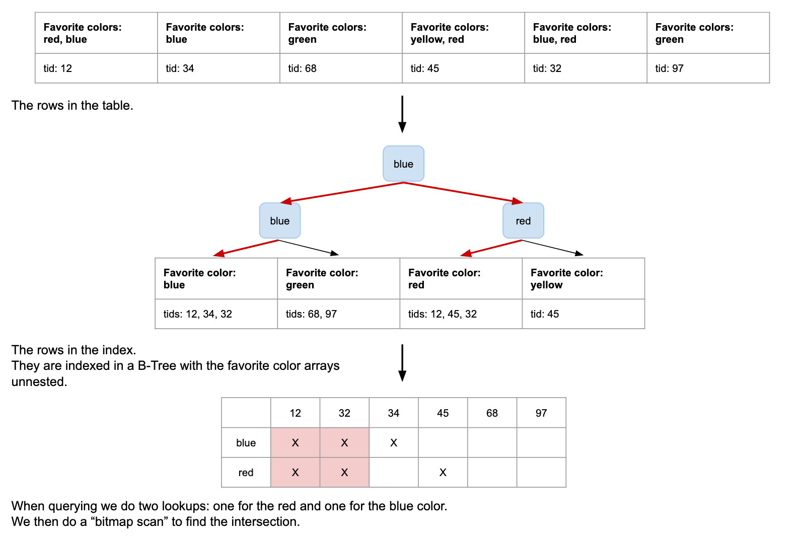
TLDR
- GIN indexes are useful to index multi-valued columns (e.g. arrays or for full-text search).
- It makes the array operations like
&&,<@,=, or@>faster. - Unlike with B-Trees, multicolumn GIN search effectiveness is the same regardless of the columns used in the query conditions. It comes from the fact that, like for array values, GIN indexes the different columns in separate B-Trees and combines the results at querying time with a bitmap scan.
Further explanation
- http://www.louisemeta.com/blog/indexes-gin/
- https://towardsdatascience.com/how-gin-indices-can-make-your-postgres-queries-15x-faster-af7a195a3fc5
- https://www.postgresql.org/docs/13/gin-implementation.html
GiST (Generalized Inverted Seach Tree)
Usecase
Ok let’s sum it up:
- Hash indexes only support the
=operator. - B-Trees support operators like
<,>and=. - GIN support operators like
&&,@>or<@for multi-valued column queries.
GiST indexes go one step further and allow indexation of complex custom operators: geospacial queries for example.
Let’s add two location_lat and location_lon columns to our users:
ALTER TABLE user ADD COLUMN location_lat FLOAT8, ADD COLUMN location_lon FLOAT8;
We want to be able to index a query that returns all the users in a 1km diameter circle around a point. Let’s say (45.7640, 4.8357):
SELECT COUNT(*)
FROM user
WHERE earth_box(ll_to_earth(45.7640, 4.8357), 1000)
		@> ll_to_earth(location_lat, location_lon)
AND earth_distance(
		ll_to_earth(45.7640, 4.8357),
		ll_to_earth(location_lat, location_lon)
	) < 1000;
Ok this looks much more complicated than what we did before 😄. What are ll_to_earth, earth_box and earth_distance?
ll_to_earth(FLOAT8, FLOAT8) -> EARTHis a function that converts coordinates to anEARTHtype.The
EARTHtype is a variation of theCUBEtype, forcing theCUBElocation to be close to the surface of the Earth.The
CUBEtype represents a shape in space. It can be a point, a line, a cube… It is efficiently indexable with GiST.earth_box(EARTH, FLOAT8) -> CUBEis a function that takes anEARTHpoint, a radius, and returns a box containing at least all the points at aradiusdistance of theEARTHpoint.This box contains too much so we need to double check the results. We refilter the results using
earth_distance(EARTH, EARTH) -> FLOAT8that returns the precise distance between twoEARTHpoints.
Ok let’s index this. We now create a GiST index on the ll_to_earth values:
CREATE INDEX user_by_location ON user
USING GIST (ll_to_earth(location_lat, location_lon));
How does it work
What makes GiST special is that it is not a kind of index per say but more of an infrastructure with a flexible/extensible api allowing complex objects to be sorted and manipulated in a search tree: geometric shapes for example. GiST can implement different indexing strategies.
In our example, we’re indexing CUBE objects, and particularly this clause:
WHERE earth_box(ll_to_earth(45.7640, 4.8357), 1000)
      @> ll_to_earth(location_lat, location_lon)
This is how our index looks like. Looks familiar?
In a B-Tree, the values of the left and right children of a node are respectively smaller and larger than their parent’s value.
In this GiST index, every node is a box with children indicating if they contain or not the points we’re looking for.
TLDR
- GiST indexes are useful in particular to index complex objects like geometric shapes.
- If we think about geometrical operations, it makes the operations like
&&,<@or@>faster for these objects, but also all the other crazy operators that can be found here. - Like with B-Trees, multicolumn GiST search is only really efficient when the query conditions match the index columns order.
Further explanation
- https://gist.github.com/norman/1535879
- https://www.postgresql.org/docs/13/cube.html
- https://www.postgresql.org/docs/13/earthdistance.html
- https://jlrobins.github.io/2019/05/simple-spatial-postgres-sans-postgis.html
- https://medium.com/postgres-professional/indexes-in-postgresql-5-gist-86e19781b5db
- http://patshaughnessy.net/2017/12/15/looking-inside-postgres-at-a-gist-index
BRIN (Block Range Indexes)
Usecase
Typically, the usecase would be for a log or audit table that is hundreds of millions of rows large:
CREATE TABLE log (
  log_entry  TEXT,
  created_at TIMESTAMP
);
We would sometimes want to query our entries by timestamp to process it for example:
SELECT COUNT(*) FROM log WHERE created_at > '2020-11-04 22:17:35'
We could definitely use a B-Tree for that. The problem is that on a table this big, the index would be multiple GB large. It would take a lot of unnecessary space in memory for such a specific background job usecase.
BRIN would be the solution. We create the index:
CREATE INDEX log_by_created_at ON log USING BRIN (created_at);
How does it work
BRIN is a special one: it doesn’t allow any new fancy complex operator indexation (only basics like <, >, =) but its structure is different.
Remember when we said that a B-Tree index was a linked list of tids, sorted by value and linked to a B-tree?
What if the data of our table was already sorted on the disk in the first place? Couldn’t we use it directly instead of having to remap the entire table as a sorted linked list for the index?
That’s exactly what BRIN is about.
Without going into details, as long as we only append to our log table (no updates, we only insert new log entries), we know that our rows will be sorted by created_at timestamp on the disk.
To index the data, BRIN will split the whole table into blocks, calculating for each the max/min values of the created_at timestamp.
The index allows us to scan the blocks instead of the rows. Let’s run our query:
SELECT COUNT(*) FROM log WHERE created_at > '2020-11-04 22:17:35'
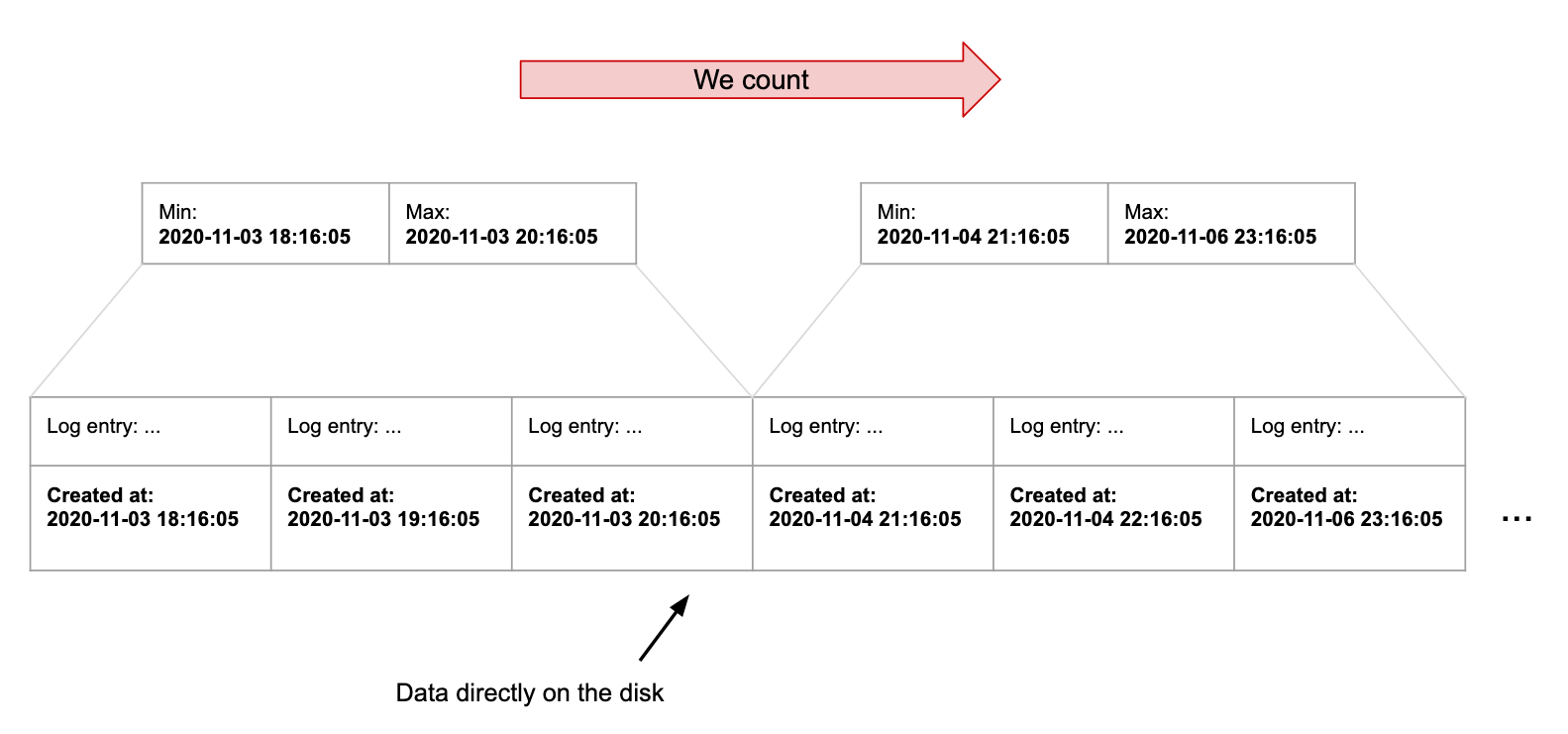
The fact that we don’t need to copy all the rows into the index makes it extremely lightweight: a few kilobytes only instead of megabytes or gigabytes for large B-Trees.
TLDR
- BRIN indexes are useful in particular to index very large append-only tables where the order of insertion is the same as the order you want to use to query.
- If your table can fit these pretty strict requirements, BRIN works well for
<,>,=operations and is extremely lightweight. - Something worth knowing is that the index only gets refreshed at vacuuming time (vacuuming is an internal Postgres garbage collection operation). To make sure that it’s refreshed before running a query you can trigger it manually by running
SELECT brin_summarize_new_values ('log_by_created_at');
Further explanation
- https://www.percona.com/blog/2019/07/16/brin-index-for-postgresql-dont-forget-the-benefits
- https://www.postgresql.org/docs/13/brin-intro.html
Conclusion
That’s all Folks!
Many people write SQL queries regularly but I noticed that many also don’t know about indexes or only ever used them as black boxes.
It is very understandable as articles and blog posts on indexes are often extremely thorough and technical (multiple pages per type of index) and it can be hard to extract general knowledge from them.
I hope that I could help with that. It was my first blog post ever and I also hope that I’ll be able to find the energy to write some more 😄.